Large Mask Development¶

Initial Resonator Design¶

Background¶

I began designing this mask with the individual resonators. There were four general design constraints. The resonators must:

Be roughly 1 mm² in size. With our roach maxed out at 250 channels this would provide appropriate coverage.
Not extend further than ∼ 400 μm from the feedline. So as not to interfere with the charge collection or overall capacitance. This is roughly the iZIP geometry.
Resonate between 3 and 3.5 GHz with a quality factor of 5 x 10⁴. The frequencies are constrained from below by our roach. As for $Q_f$ , we want something closer to 10⁴ but from experience we know that actual $Q_f$ is roughly a factor of five lower than simulation.

Design, tuning and results¶

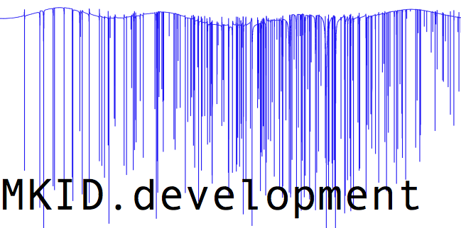
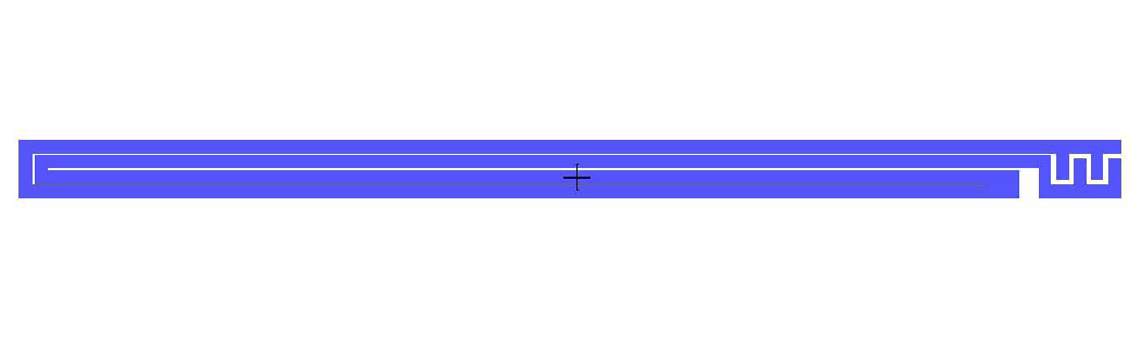
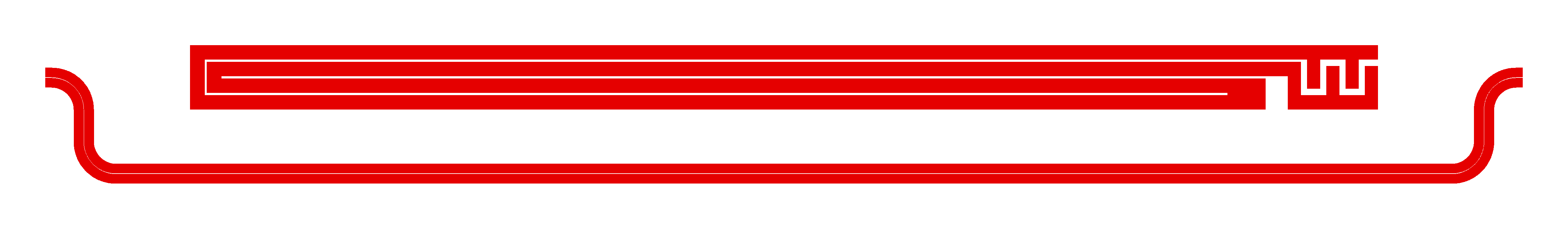
Using these as a starting point I settled on a “fold over” form factor:

This basic design is both narrow and (in the far field) nowhere a dipole.

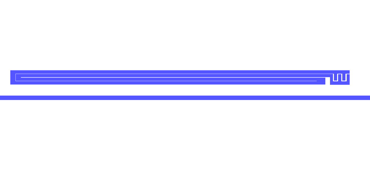
With this basic design, I used an internal port and measured the input impedance at this port over a wide frequency range (Jiansong’s method ).

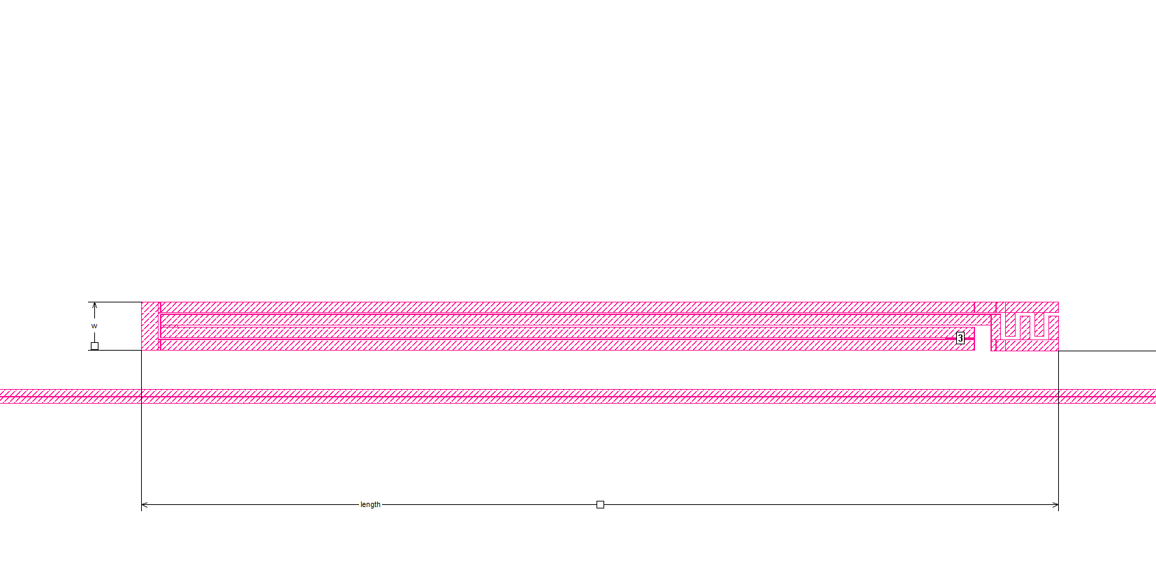
The placement of the third port in Sonnet

After the third port is was in place, I ran a suite of simulations and sort of heuristically converged on an optimal design by looking at the input impedance of the third port.

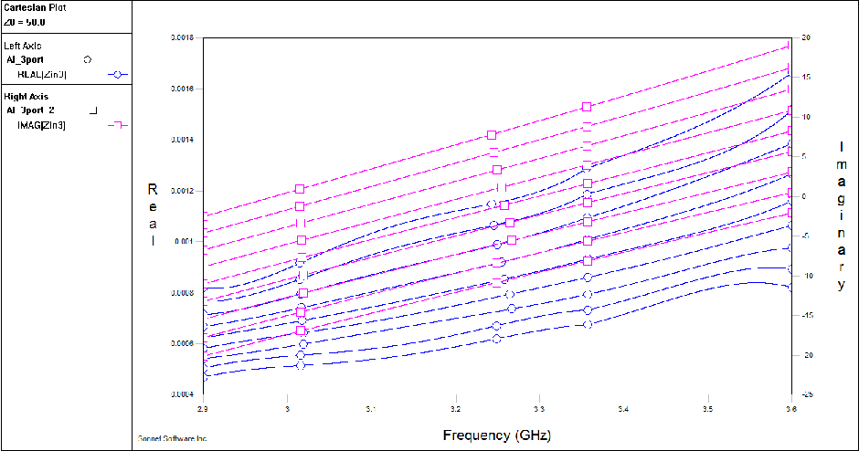
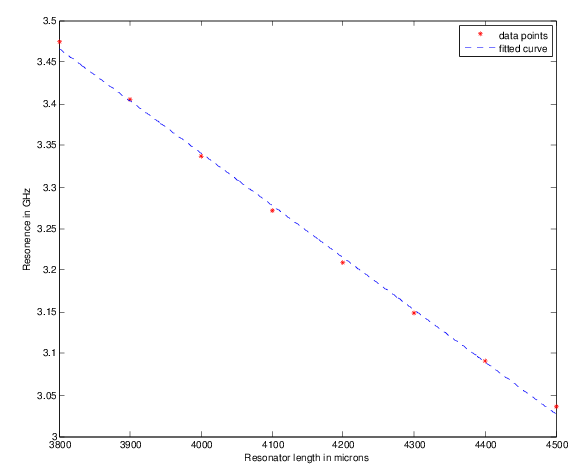
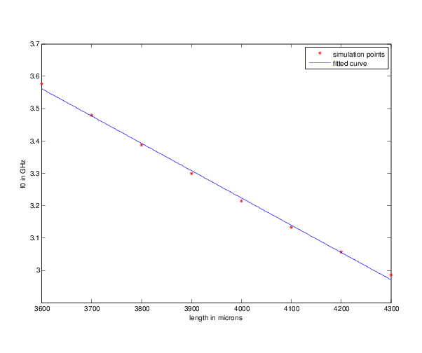
After much tuning, this is the response for sweeps at various inductor lengths.

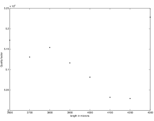
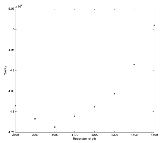
After tuning for the correct $Q_f$ I was able to get quite a nice comb of resonances just by varying the length of the inductive meander. A graph of the response vs length is nicely linear and the quality factors change by less than 3%.

Resonant frequencies and linear fit	Quality factor

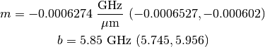
I have fit this responce them to a linear form

$f(x) = mx + b$

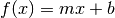
resulting in coefficients (and 95% confidence bounds) of

$m = -0.0008433~ \frac{\text{GHz}}{\text{$\mu$m}}~ (-0.0008841, -0.0008026) b = 6.598~ \text{GHz}~ (6.436, 6.759)$

As can be seen the quality factor is not strongly dependent on the resonator length over this range (it is not even monotonic). As a result I will not worry about varying the distance from the resonator to the feedline; I will only vary the length.

Python gdspy.cell object¶

The object¶

I coded up a function in python (see Source) using the gdspy module that generates a resonator of whatever length I desire.

My gdspy.cell resonator

Gdspy.cell Simulations¶

Because this was coded, not hand made and extensively tuned (like the prototype discussed earlier), its dimensions are nice even numbers. This required very slight changes in the geometry of the device (on order of one micron here and there). As a result, I wanted to re-run my simulations on it to see how its behaviour has changed. The results are plotted in figure 5 and the fit has a slope and intercept of:

$m = -0.0006274~ \frac{\text{GHz}}{\text{$\mu$m}}~ (-0.0006527, -0.000602) b = 5.85~ \text{GHz}~ (5.745, 5.956)$

Clearly the slope of this resonator response curve is strongly dependent on the resonator geometry (the small changed produced by automation reduced m by a factor of 25%). The quality factors are largely unaffected though, and the resonator is clearly still usable.

Resonant frequencies for gdspy.cell	Quality factor for gdspy.cell

Current distribution¶

Finally, I took a look at the current distribution in the inductor.

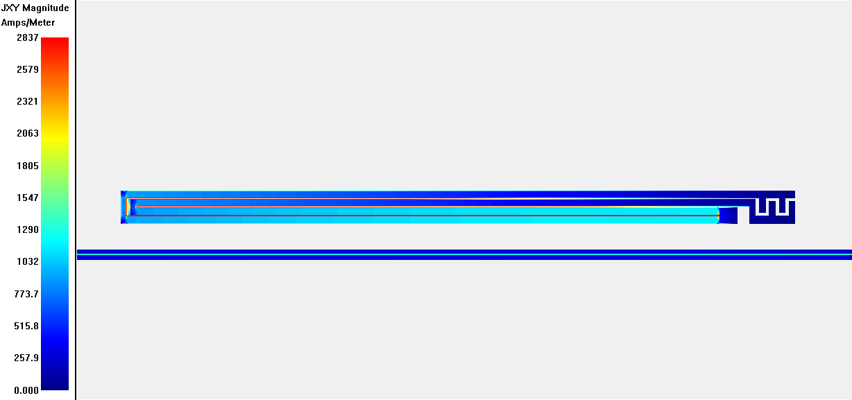
The current density of the resonator

I also calculated the efficiency ξ of our inductor which is the ratio of the measured current (the integral of the blue line in the figure) to the theoretical maximum current (the dotted red line–note: I have not convinced myself this is a valid way of doing this) or:

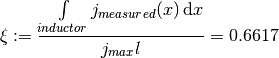
$\xi := {\int\limits_{inductor} j_{measured}(x)\, \mathrm{d}x \over j_{max} l} = 0.6617$

Which is just the ratio of the area under the blue curve and red dotted line below.

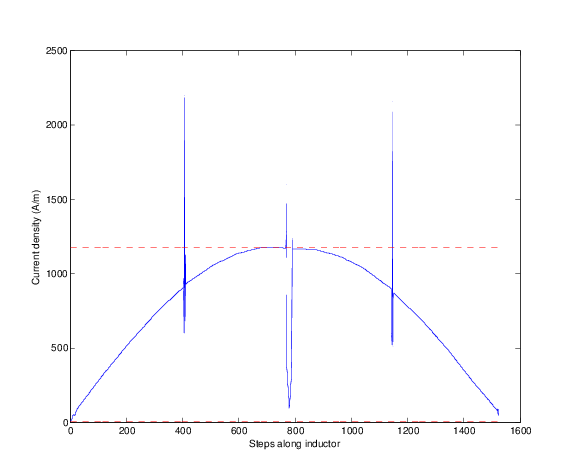
The blue is the measured current density. The red is the max (excluding aberrations on the boundaries)

Bent feedline¶

In an attempt to minimize the capacitance between my phonon channel and my charge channel, I tried to keep center of mass of my resonator and feedline combination centered between the charge rails. This requires a bend in the feedline; between resonators the feedlines should be centered, but when it encounters a resonator, it needs to bend to account for the resonators mass. This lead to an initial design that looked like this:

This is my first attempt at a bent feedline (source bent-feedline-source)

The next course of action was to simulate this is sonnet to see how close I can get the bend to the resonator without degrading the quality. This first attempt had the straight segment 1.125 times the length of the resonator and it did not significantly impact the quality ( $Q_f = 48,051$ ). I will simulate at a few more lengths, but this design seems like it will work.

Initial Mask Design¶

My initial mask design ditched the bent feedline in favor of a simpler polygon based design:

This is my initial mask design. Due to the relatively tight angular spacing of the resonators the capacitance should not be overly effected by the lack of a bend.

Coupling Simulations¶

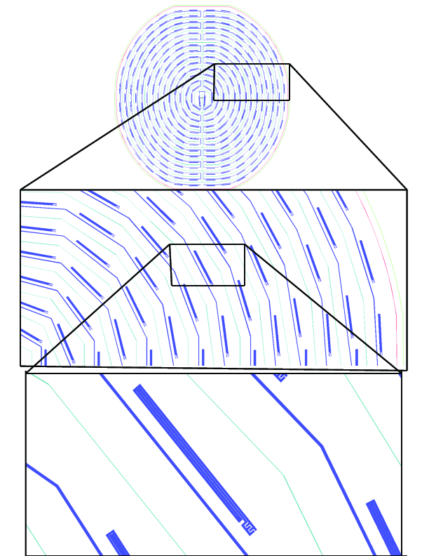
With the basic layout of the mask decided, I needed to simulate the cross couplings. I was most concerned about radial coupling (especially for the resonators that fully overlapped at 6 and 12). My initial simulations were of a pair of resonators from the vertical axis of the device and I found very little evidence of coupling as can be seen in this current simulation:

As can be seen, during the resonance of the lower MKID there is no current in the upper MKID.

There was also no frequency shift of the lower resonator when the upper MKID was removed. This being said, the lower resonator was not operating at its design frequency; there was some unwanted feedline coupling. To get a handle on this I did a number of parameter sweeps of the vertical and horizontal (g2 and g1 in the figure below) separation between the lower MKID and the feedline.

Parameter sweeps to understand the coupling to the feedline.

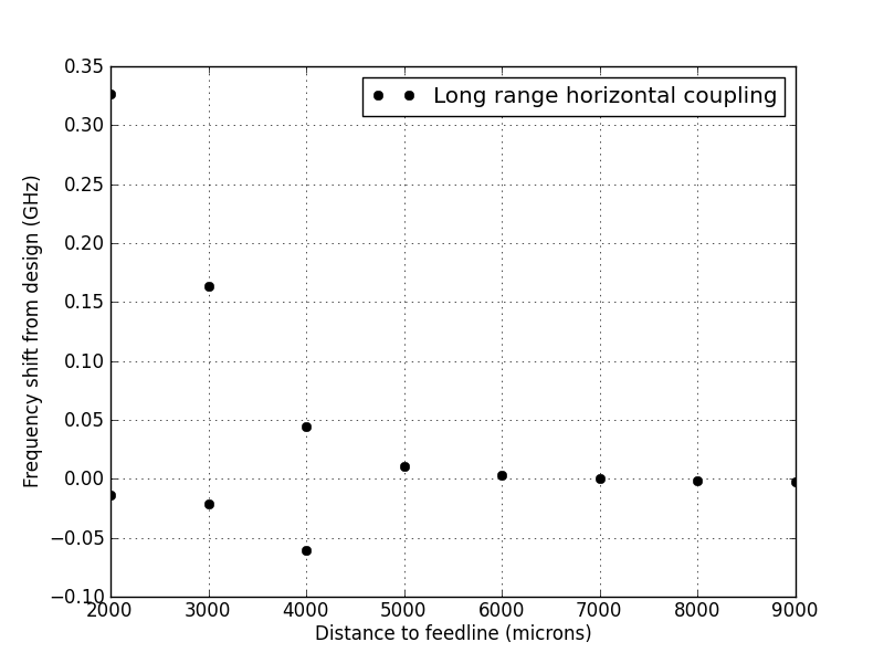
Which resulted in the following shifts in the design frequency.

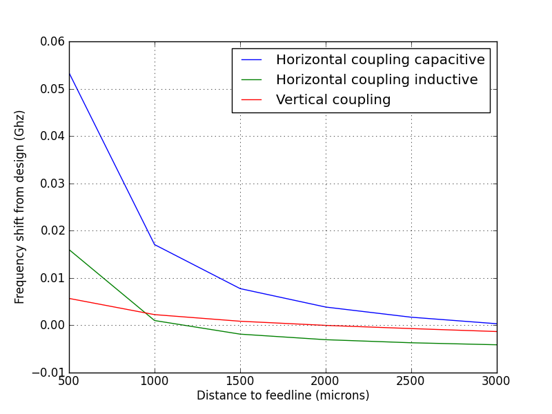
The frequency shift resulting from both vertical and horizontal parameter sweeps of the feedline.

This effect is not ideal, but it can be measured and corrected for. The negative frequency shift is a little confusing. One would expect, in the limit of large spacings, that the design frequency would be recovered. This could be explained by some kind of two regime thing where the short range couplings strongly decrease the capacitance, but there is also a weaker increase of the inductance that is only visible at longer distances after the capacitive coupling has dropped off. I did a simulation of this limit in the vertical direction (as seen below) and

This was my sanity check geometry for the previous simulations.

This parameter sweep produced the following results:

The change in resonant frequency from the design frequency. It appears that there may be multiple resonances produced in the 500 MHz of bandwidth that I observe. This may take more though to design around.

It appears that part of what I am seeing is a secondary resonance, and that the primary is what have been observing all along. I am not sure If this will be a problem as it seems that the secondary can be designed around. My main concern would be a situation where a single resonator would have two resonances in the 3 to 3.5 GHz range that I will be probing.

As a last step I did a couple of coupling simulations in the angular direction. I did a parameter sweep of horizontal resonator simulations as a first run through and observed frequency shifts on the order of a few kHz and no sign of coupling from the current simulations.

This is a current simulation showing no coupling even for an unrealistically small separation (500 microns).

To do this correctly I should probably do a voided crossing simulation, but given my explicit control of the frequency spacing of resonators in this direction this is enough to convince me to pay more attention at the feedline coupling problem.

Coupling Corrections¶

The main correction that I will do is to the resonators that have to deal with the horizontal feedline couplings (as simulated above). To do this I simulated the frequency shift experienced by a resonator that is on the vertical axis of the mask. The results are below:

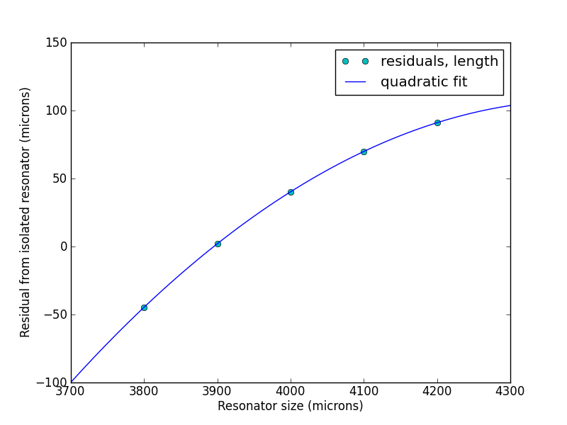
This is a quadratic fit to the residuals (isolated resonator length - true length). I will use it to correct the effected resonators.

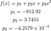
I can correct the MKIDS affected by the vertical feedline by simply subtracting this residual quantity. For ease if use I fit the points to a quadratic (no a priori reason for this...it just looked quadratic). The functional form and fit parameters are:

$f(x) = p_1 + p_2x + p_3x^2 p_1 = -812.92 p_2 = 3.7455 p_3 = -4.2579 \times 10^{-4}$

I then applied this correction to the appropriate resonators and colored them yellow (as a check to make sure I got the right ones). The results are the mask below:

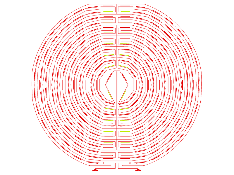
The yellow MKIDS are the ones I applied my correction to. It looks like I got them all

Source¶

Variable length resonator function source:

import gdspy

def resonator(length, name):

    #initialize cell
    poly_cell = gdspy.Cell(name)

    #variables
    indgap,capgap,width,cwidth = 7.0,20.0,45.0,40.0

    ########INDUCTOR##########

    #left vertical
    ll = (0.0, 0.0)
    ur = (width, 4.0*width + 3.0*indgap)
    poly_cell.add(gdspy.Rectangle(1, ll, ur))

    #top horizontal
    ll = (width, 3.0*width + 3.0*indgap)
    ur = (length, 4.0*width + 3.0*indgap)
    poly_cell.add(gdspy.Rectangle(1, ll, ur))

    # 2nd horizontal
    ll = (width + indgap, 2.0*width + 2.0*indgap)
    ur = (length - 5.0*cwidth - 4.0*capgap, 3.0*width + 2.0*indgap)
    poly_cell.add(gdspy.Rectangle(1, ll, ur))

    # 3rd horizontal
    ll = (width + indgap, 1.0*width + 1.0*indgap)
    ur = (length - 5.0*cwidth - 4.0*capgap - 70.0, 2.0*width + 1.0*indgap)
    poly_cell.add(gdspy.Rectangle(1, ll, ur))

    # bottom horizontal
    ll = (width, 0.0)
    ur = (length - 5.0*cwidth - 4.0*capgap - 70.0, width)
    poly_cell.add(gdspy.Rectangle(1, ll, ur))

    # end connecting piece
    ll = (length - 5.0*cwidth - 4.0*capgap - 70.0 - 118.0, width)
    ur = (length - 5.0*cwidth - 4.0*capgap - 70.0, width + indgap)
    poly_cell.add(gdspy.Rectangle(1, ll, ur))

    # middle connecting piece
    ll = (width + indgap, 2.0*width + indgap)
    ur = (2.0*width + indgap, 2.0*width + 2.0*indgap)
    poly_cell.add(gdspy.Rectangle(1, ll, ur))

    ########CAPACITOR########

    # bottom horizontal
    ll = (length - 5.0*cwidth - 4.0*capgap, 0.0)
    ur = (length, width)
    poly_cell.add(gdspy.Rectangle(1, ll, ur))

    # finger one (from right)
    ll = (length - cwidth, width)
    ur = (length, 3.0*width + 3.0*indgap - capgap)
    poly_cell.add(gdspy.Rectangle(1, ll, ur))

    # finger three (from right)
    ll = (length - 3.0*cwidth - 2.0*capgap, width)
    ur = (length - 2.0*cwidth - 2.0*capgap, 3.0*width + 3.0*indgap - capgap)
    poly_cell.add(gdspy.Rectangle(1, ll, ur))

    # figner five (from right)
    ll = (length - 5.0*cwidth - 4.0*capgap, width)
    ur = (length - 4.0*cwidth - 4.0*capgap, 3.0*width + 3.0*indgap - indgap)
    poly_cell.add(gdspy.Rectangle(1, ll, ur))

    # figer two (from right)
    ll = (length - 2.0*cwidth - 1.0*capgap, width + capgap)
    ur = (length - 1.0*cwidth - 1.0*capgap, 3.0*width + 3.0*indgap)
    poly_cell.add(gdspy.Rectangle(1, ll, ur))

    # finger four
    ll = (length - 4.0*cwidth - 3.0*capgap, width + capgap)
    ur = (length - 3.0*cwidth - 3.0*capgap, 3.0*width + 3.0*indgap)
    poly_cell.add(gdspy.Rectangle(1, ll, ur))

    return poly_cell

The source for the resonator with the bent feedline:

import os
import gdspy
from newres import resonator

def bend(length, feedline):
    """
    This adds a bend (for going around the resonator) wih a lenght of length
    """
    feedline.segment(1, 20)
    feedline.turn(1,100,'r')
    feedline.segment(1,100,)
    feedline.turn(1, 100, 'l')
    feedline.segment(1,1.125*length)
    feedline.turn(1, 100, 'l')
    feedline.segment(1,100)
    feedline.turn(1,100,'r')
    feedline.segment(1, 20)
    return feedline

#initialize cell object
raf_cell = gdspy.Cell('RAF')

#initialize path object and add a bend and add it to the cell
feedline = gdspy.Path(30.0, (0., 0.),number_of_paths=2, distance=32.0)
feedline = bend(3700., feedline)
raf_cell.add(feedline)

#add a resonator
res = resonator(3700.,'RES')
raf_cell.add(gdspy.CellReference(res,(220.+.0625*3700.,-100)))

gdspy.gds_image(cells='RAF', background=(255, 255, 255)) #saves a .png

## Create the full file name to save the GDSII layout.
name = os.path.abspath(os.path.dirname(os.sys.argv[0])) + os.sep +\
   'RAF'

## Output the layout to a GDSII file (default to all created cells).
## Set the units we used to micrometers and the precision to nanometers.
gdspy.gds_print(name + '.gds',cells=[raf_cell], unit=1.0e-6, precision=1.0e-9)
print 'Sample gds file saved: ' + name + '.gds'

Table Of Contents

Previous topic

This Page

Large Mask Development¶

Initial Resonator Design¶

Background¶

Design, tuning and results¶

Python gdspy.cell object¶

The object¶

Gdspy.cell Simulations¶

Current distribution¶

Bent feedline¶

Initial Mask Design¶

Coupling Simulations¶

Coupling Corrections¶

Source¶

Navigation

Table Of Contents

Previous topic

This Page

Quick search

Large Mask Development¶

Initial Resonator Design¶

Background¶

Design, tuning and results¶

Python gdspy.cell object¶

The object¶

Gdspy.cell Simulations¶

Current distribution¶

Bent feedline¶

Initial Mask Design¶

Coupling Simulations¶

Coupling Corrections¶

Source¶

Navigation